42 figures
List of figures
Every figure of the explanation with description, chapter reference and download. The numbers are taken from the thesis; they do not follow the reading order of this site.
42 of 42 figures
-
Fig. 1
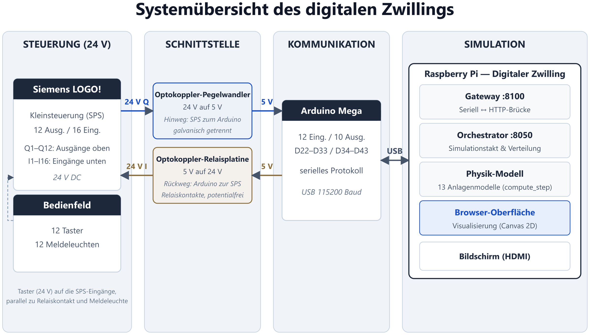
System overview
Four levels from the controller to the simulation: Siemens LOGO! (24 V), converter stages, Arduino Mega as signal bridge, Raspberry Pi with gateway, orchestrator and physics model.
-
Fig. 2
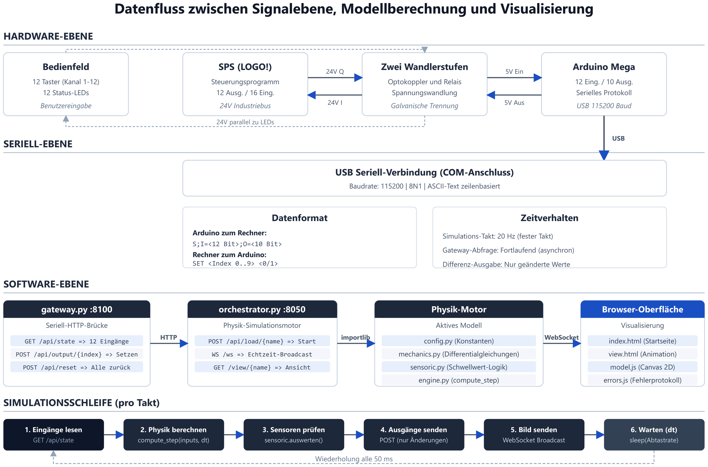
Data flow
Path of the signals from the hardware level via the model calculation to the visualisation in the browser.
-
Fig. 2a
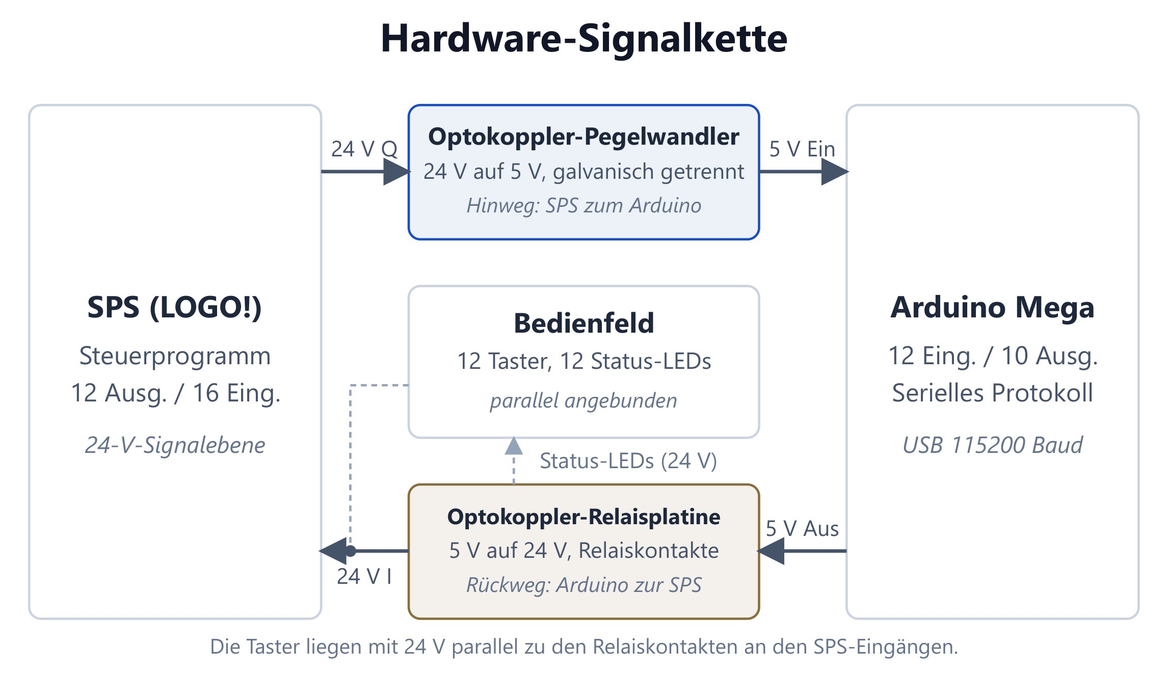
Hardware signal chain
Forward path via the optocoupler level converter, return path via the relay board; control panel connected in parallel.
-
Fig. 2b
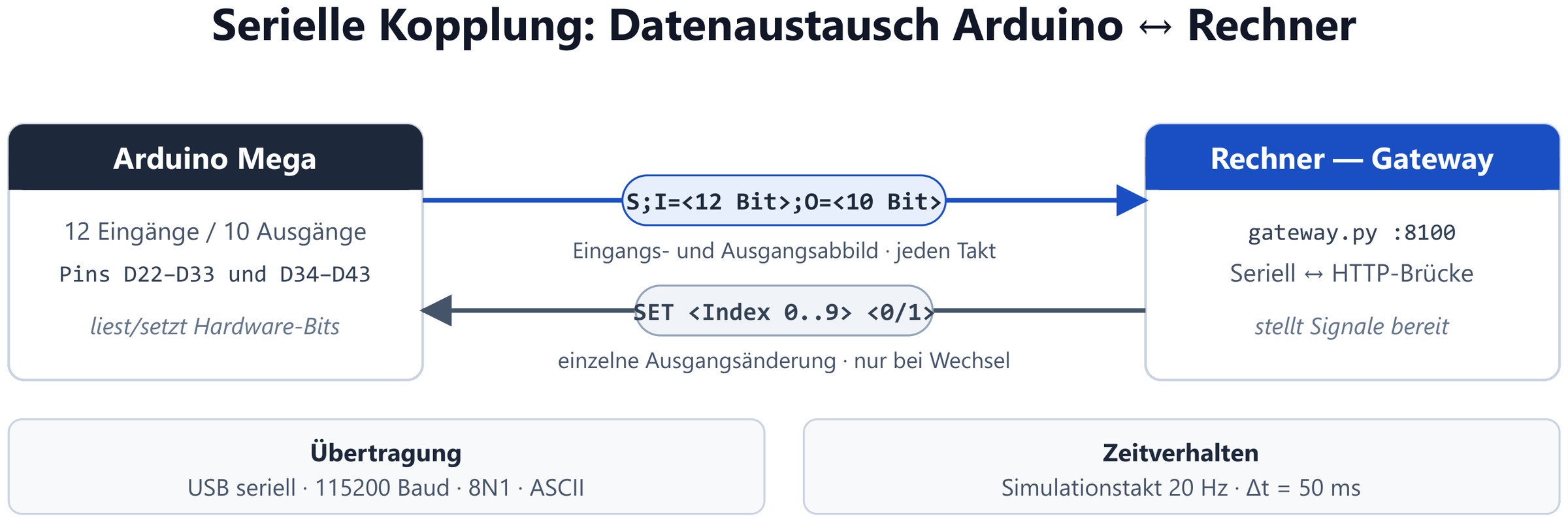
Serial data format
Structure of the telegrams between Arduino Mega and gateway (USB, 115200 baud).
-
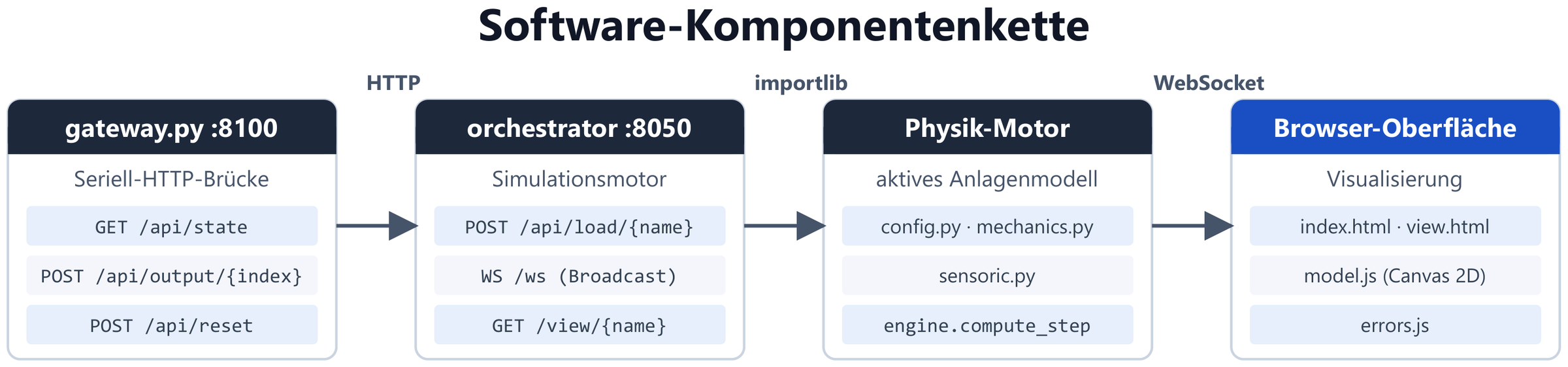
Fig. 2c
Software component chain
gateway.py (:8100) as serial-HTTP bridge, orchestrator.py (:8050) as simulation engine, below it the active plant model.
-
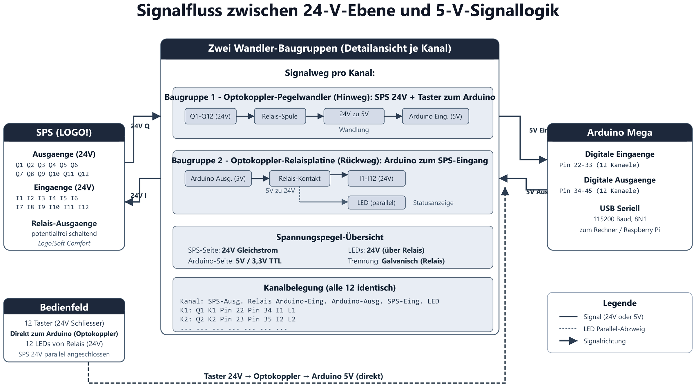
Fig. 3
Signal flow 24 V / 5 V
Channel-by-channel assignment of the controller outputs Q1–Q12 and inputs I1–I16 to the 5 V signal logic.
-
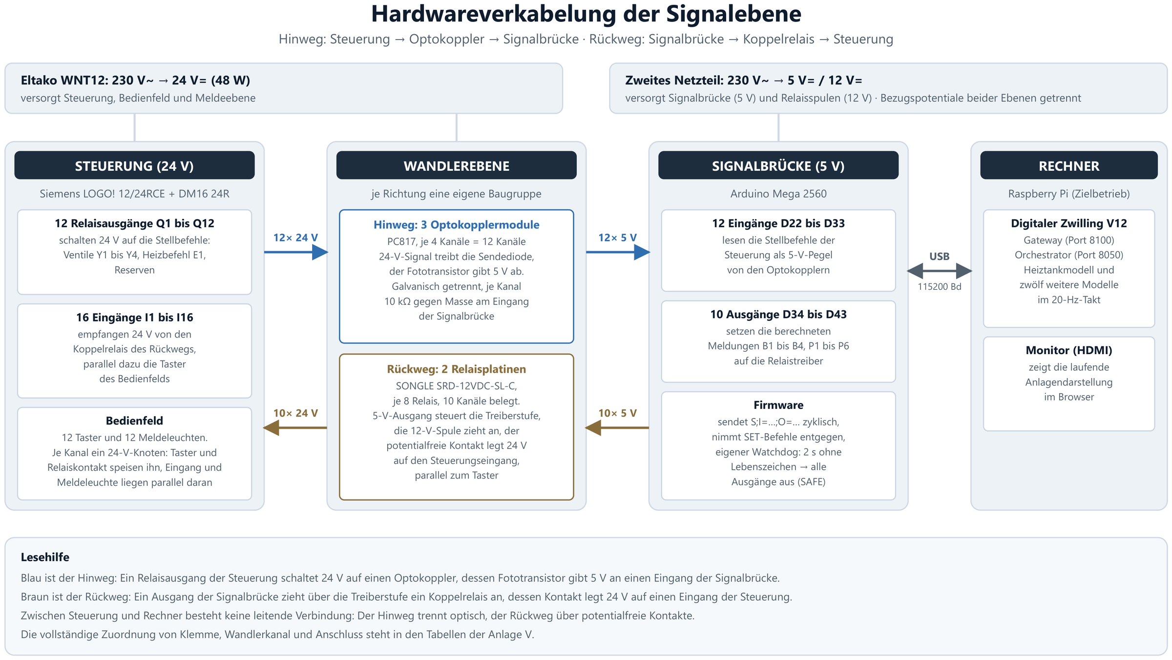
Fig. 4
Hardware cabling
Power supplies, reference potentials and wiring of the signal level: 230 V → 24 V for the controller, 5 V and 12 V for signal bridge and relay coils.
-
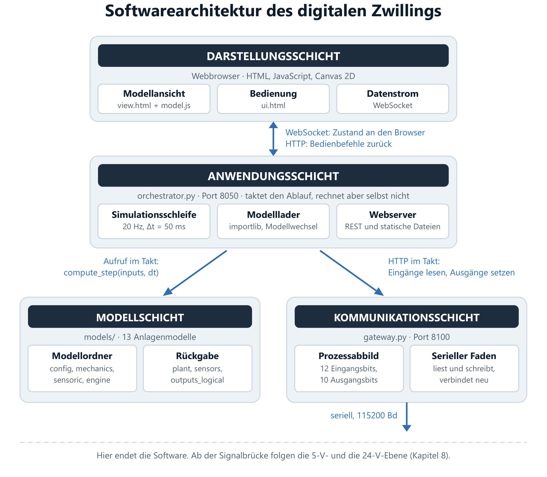
Fig. 5
Software architecture (simplified)
Three layers: presentation in the browser, application in the orchestrator, communication in the gateway.
-
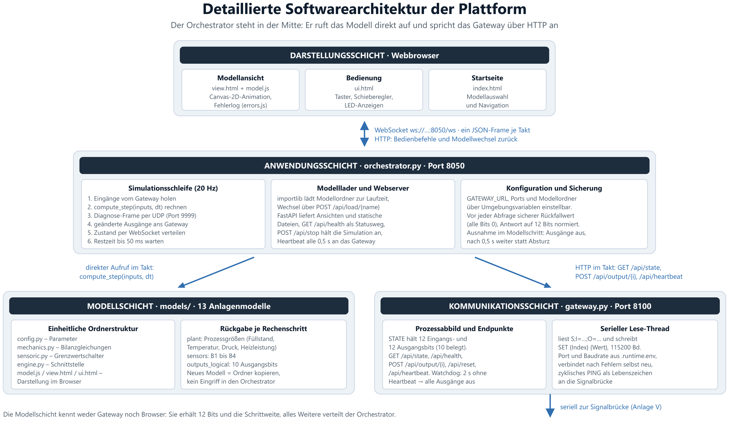
Fig. 5
Software architecture (detailed)
The orchestrator in the middle: it calls the model directly and addresses the gateway via HTTP.
-
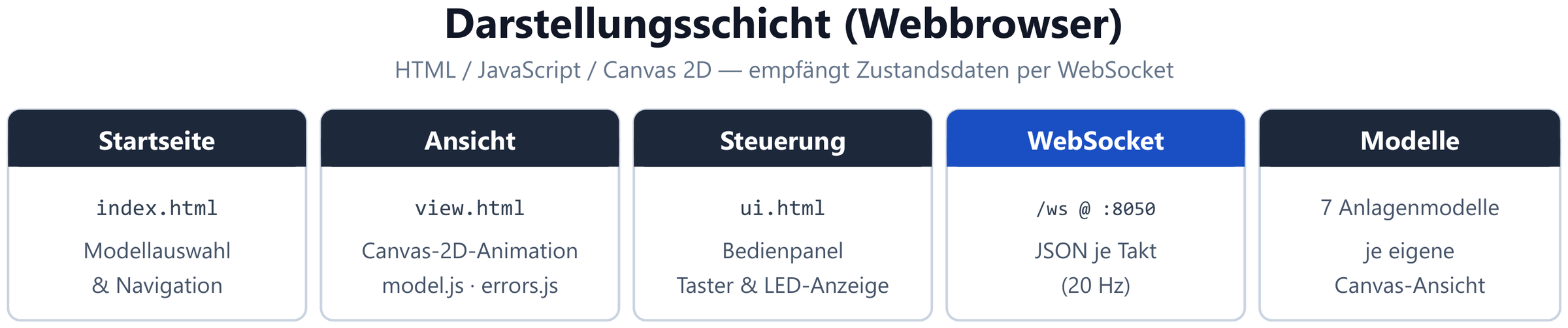
Fig. 5a
Presentation layer
Browser with Canvas 2D animation, operating panel and error log; state data arrives every cycle via WebSocket.
-
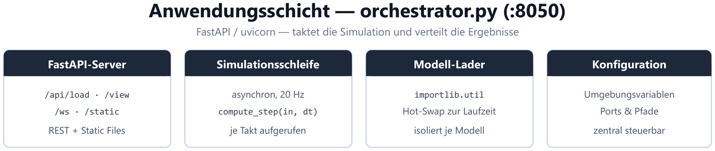
Fig. 5b
Application layer
orchestrator.py: FastAPI server, asynchronous simulation loop at 20 Hz, model loader with hot swap at runtime.
-
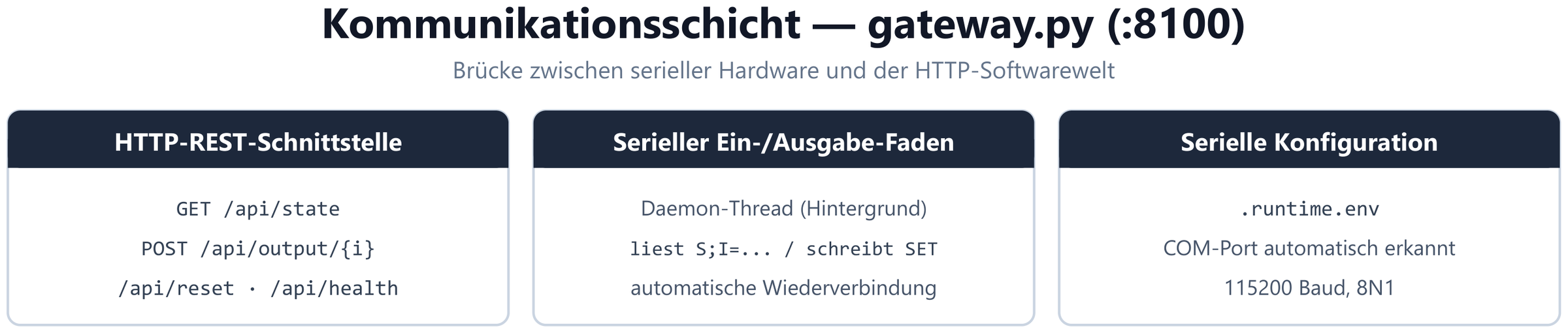
Fig. 5c
Communication layer
gateway.py as a bridge between serial hardware and HTTP: own read/write thread with automatic reconnection.
-
Fig. 5d
Physics model layer
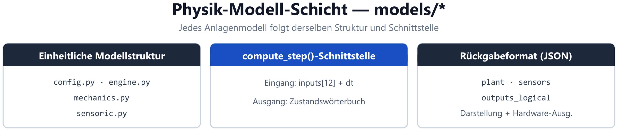
Uniform structure of every plant model: config, engine, mechanics, sensoric — addressed via compute_step(inputs, dt).
-
Fig. 6
Overview of the plant models
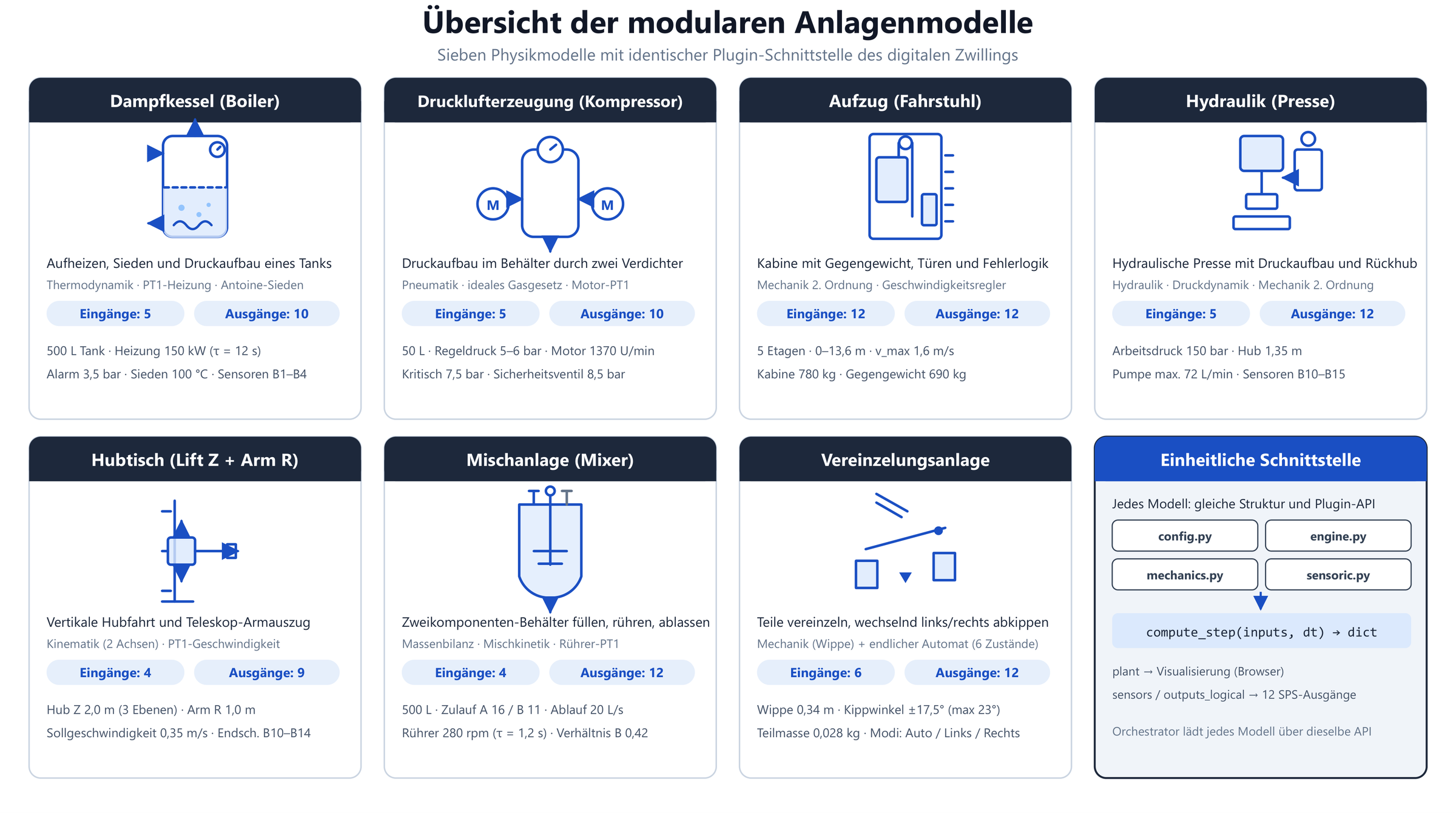
Several physics models with an identical plugin interface; the heated tank is one of them.
-
Fig. 7a
Heated-tank model, schematic
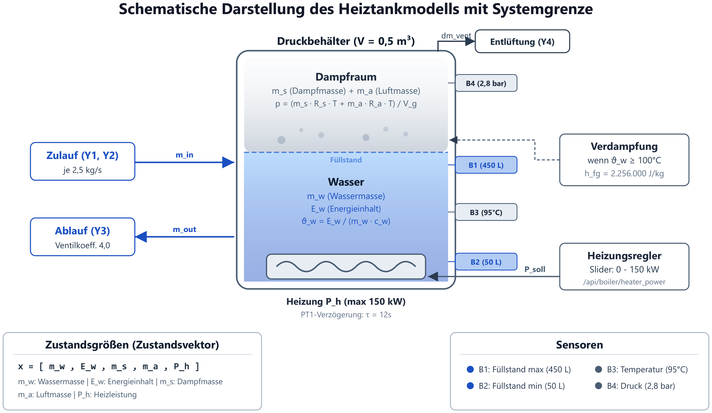
Pressure vessel of 0.5 m³, water and steam space, heater with PT1 behaviour (τ = 12 s) and the system boundary of the model.
-
Fig. 7b
Running simulation
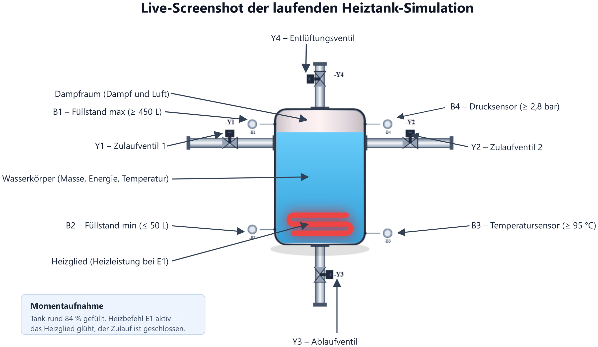
Labelled snapshot of the heated tank in operation (tank about 84 % full, heating command E1 active): water body, steam space, heating element, valves Y1–Y4 and the sensors B1–B4.
-
Fig. 8
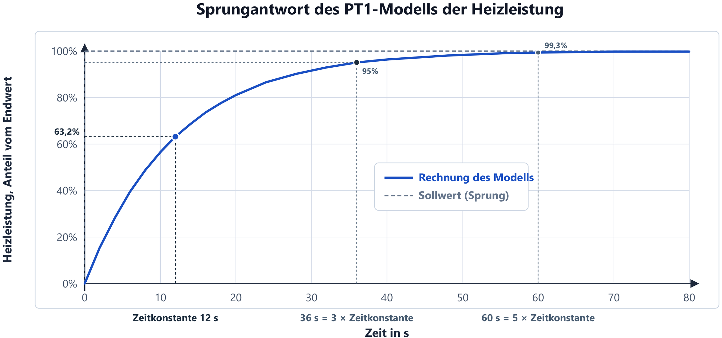
PT1 step response
Heating power after a step: 63.2 % after one time constant, 95 % after three, 99.3 % after five.
-
Fig. 9
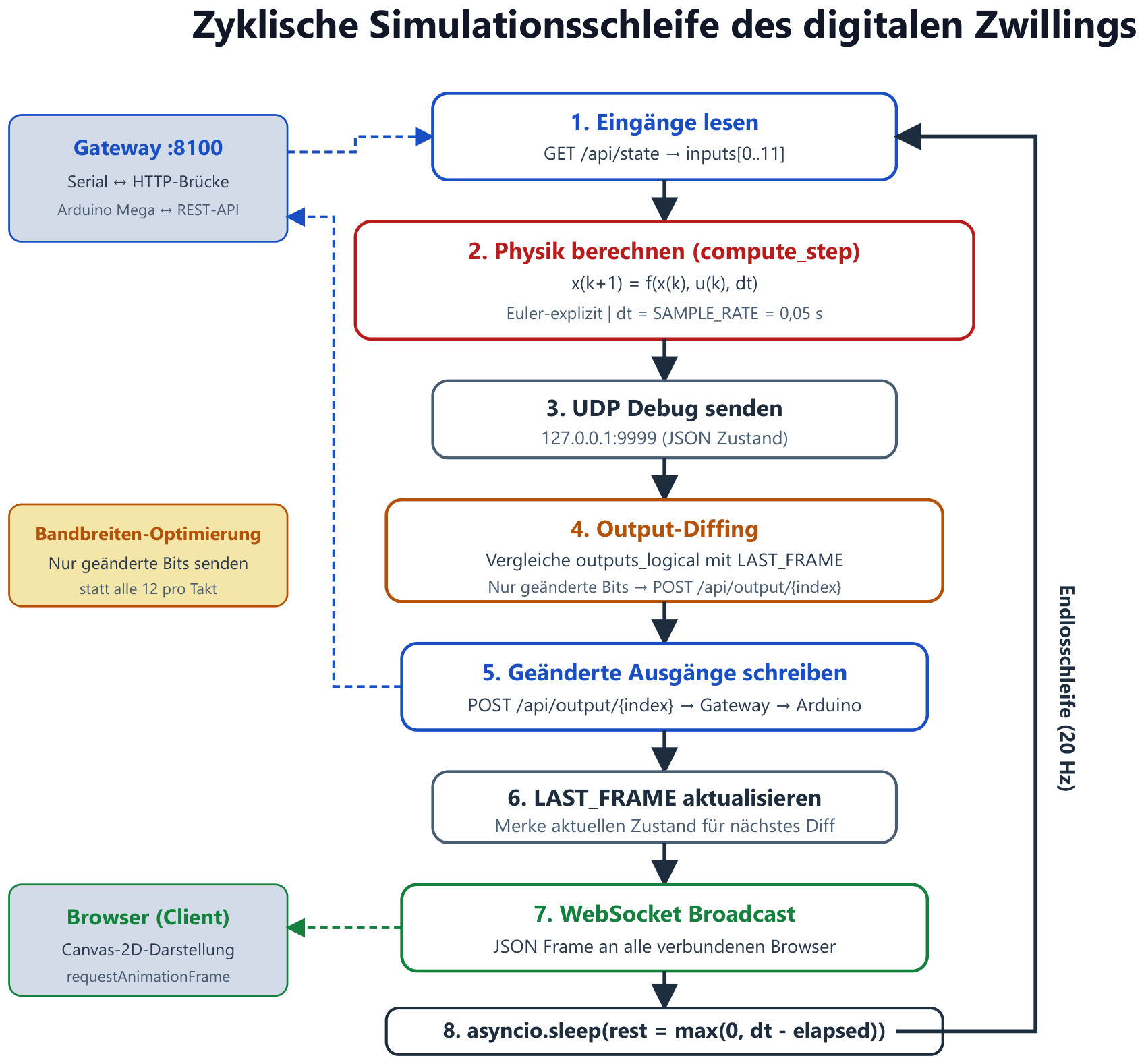
Simulation loop
One cycle of the 20 Hz loop: read inputs, calculate physics (Δt = 0.05 s), send debug, compare outputs, write changed outputs, serve browsers via WebSocket, wait out remaining time.
-
Fig. 10
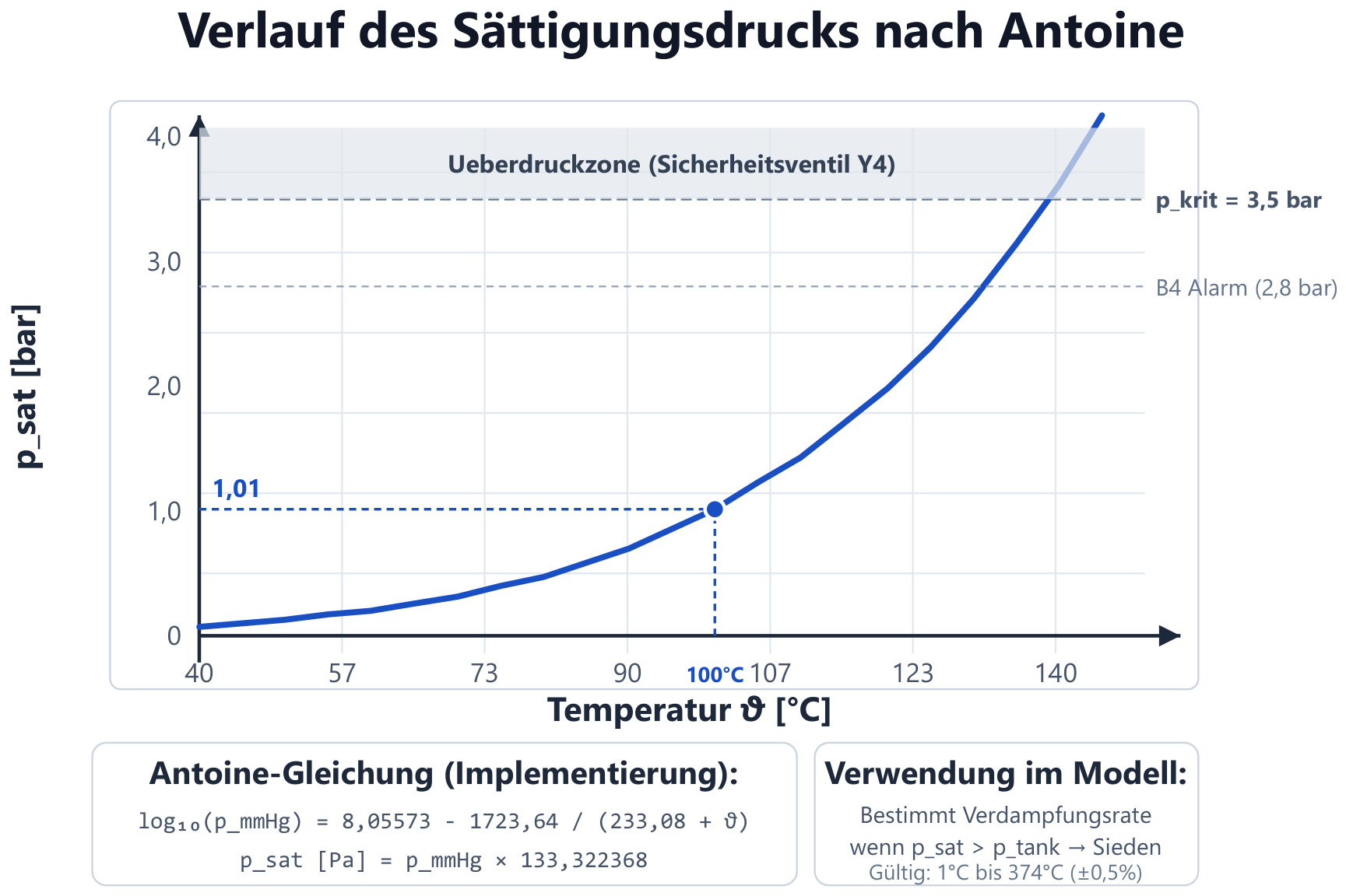
Saturation pressure according to Antoine
Curve of the saturation pressure over temperature with alarm threshold B4 (2.8 bar) and safety valve (3.5 bar).
-
Fig. 11
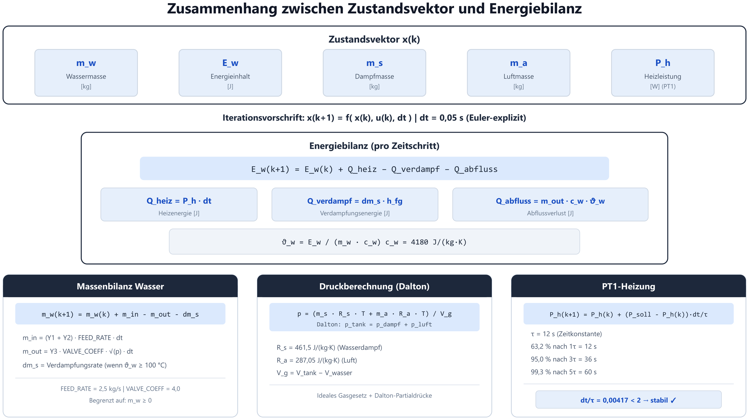
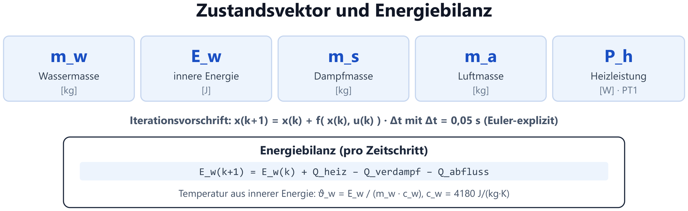
State vector and energy balance
The five state variables and their update per time step with energy balance, mass balance, pressure calculation and PT1 heating.
-
Fig. 11a
State vector
Water mass, internal energy, steam mass, air mass and heating power as the state x(k).
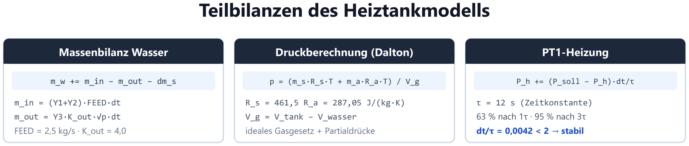
-
Fig. 11b
Partial balances
Mass balance of the water, evaporation and pressure calculation according to Dalton with the gas constants for steam and air.
-
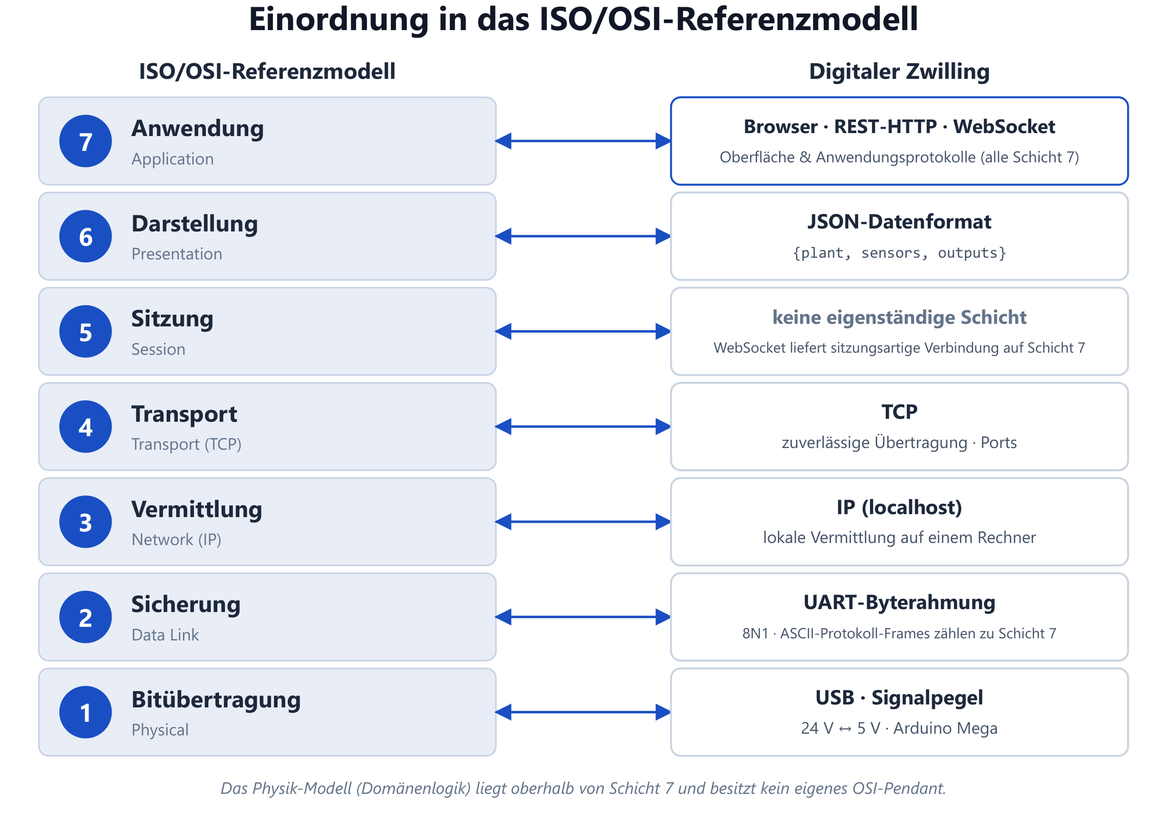
Fig. 12
Classification in the ISO/OSI model
Where browser, REST, WebSocket, JSON and the serial connection sit in the reference model.
-
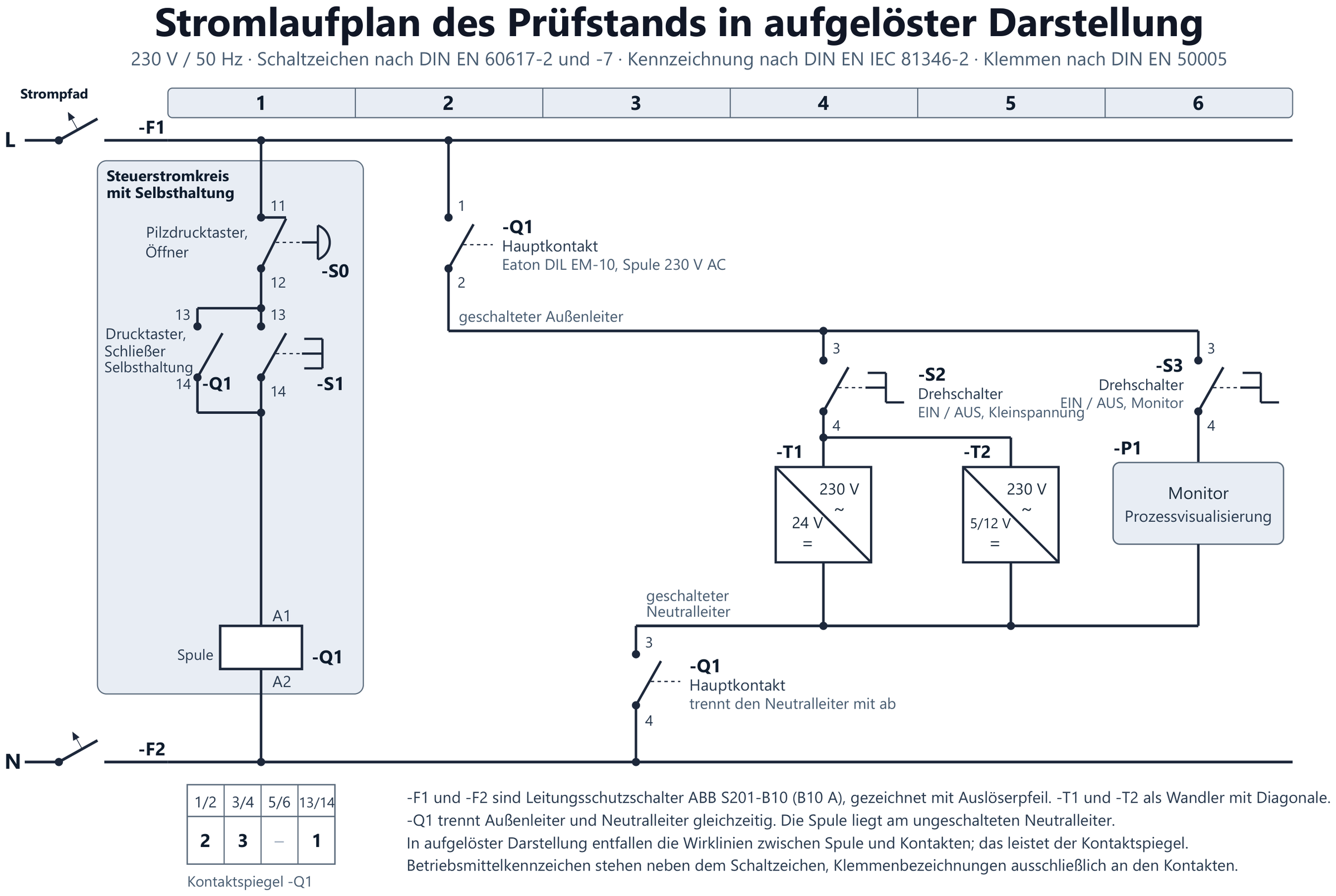
Fig. 13
Circuit diagram 230 V
Detached representation of the test rig with self-holding and emergency stop; symbols according to DIN EN 60617, designation according to DIN EN IEC 81346-2, terminals according to DIN EN 50005.
-
Fig. 14a
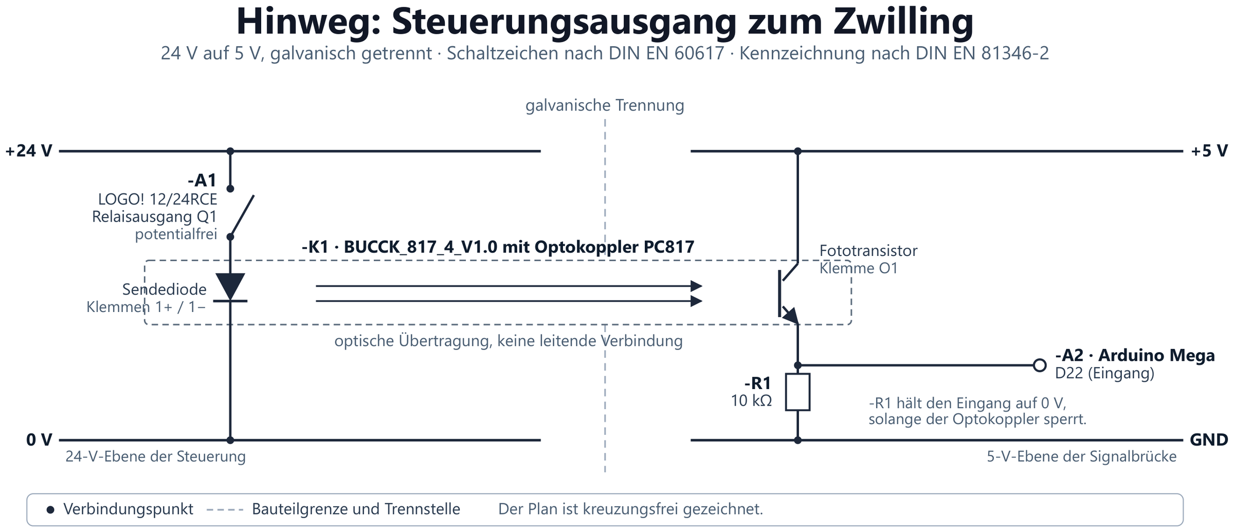
Signal path forward
24 V to 5 V via a PC817 optocoupler: optical transmission without a conductive connection.
-
Fig. 14b
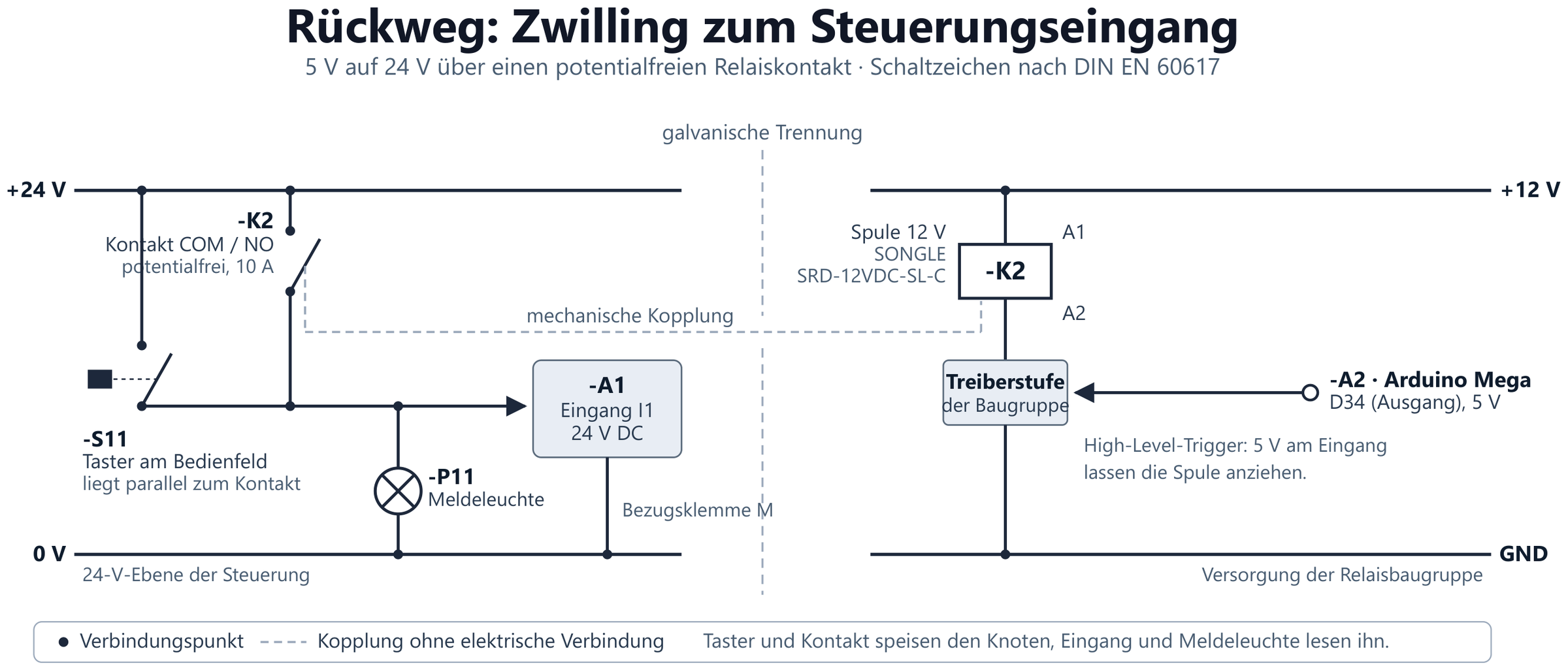
Signal path return
5 V to 24 V via a potential-free relay contact, in parallel with the push button on the control panel.
-
Fig. 15
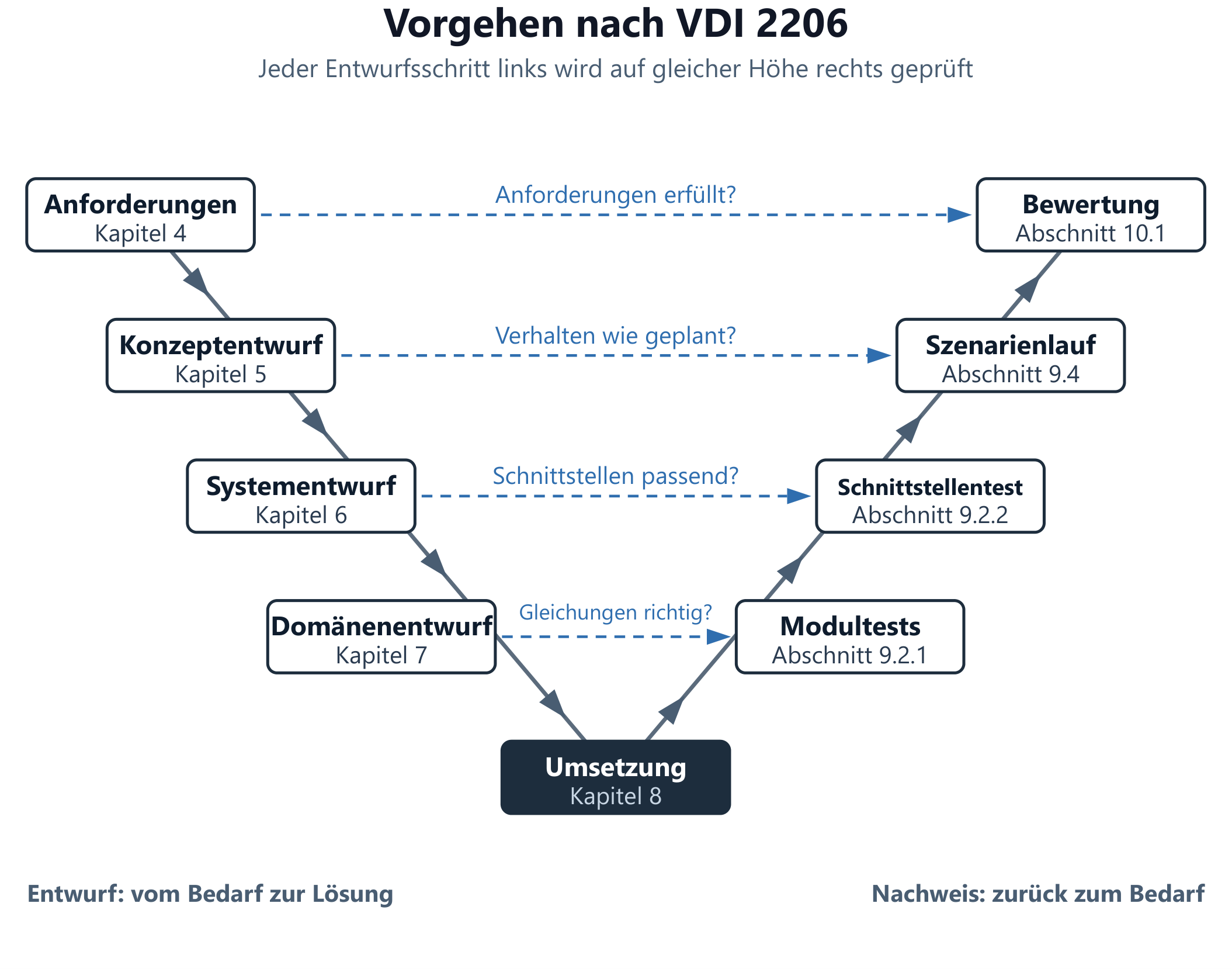
Approach according to VDI 2206
Each design step on the left is verified at the same level on the right.
-
Fig. 16
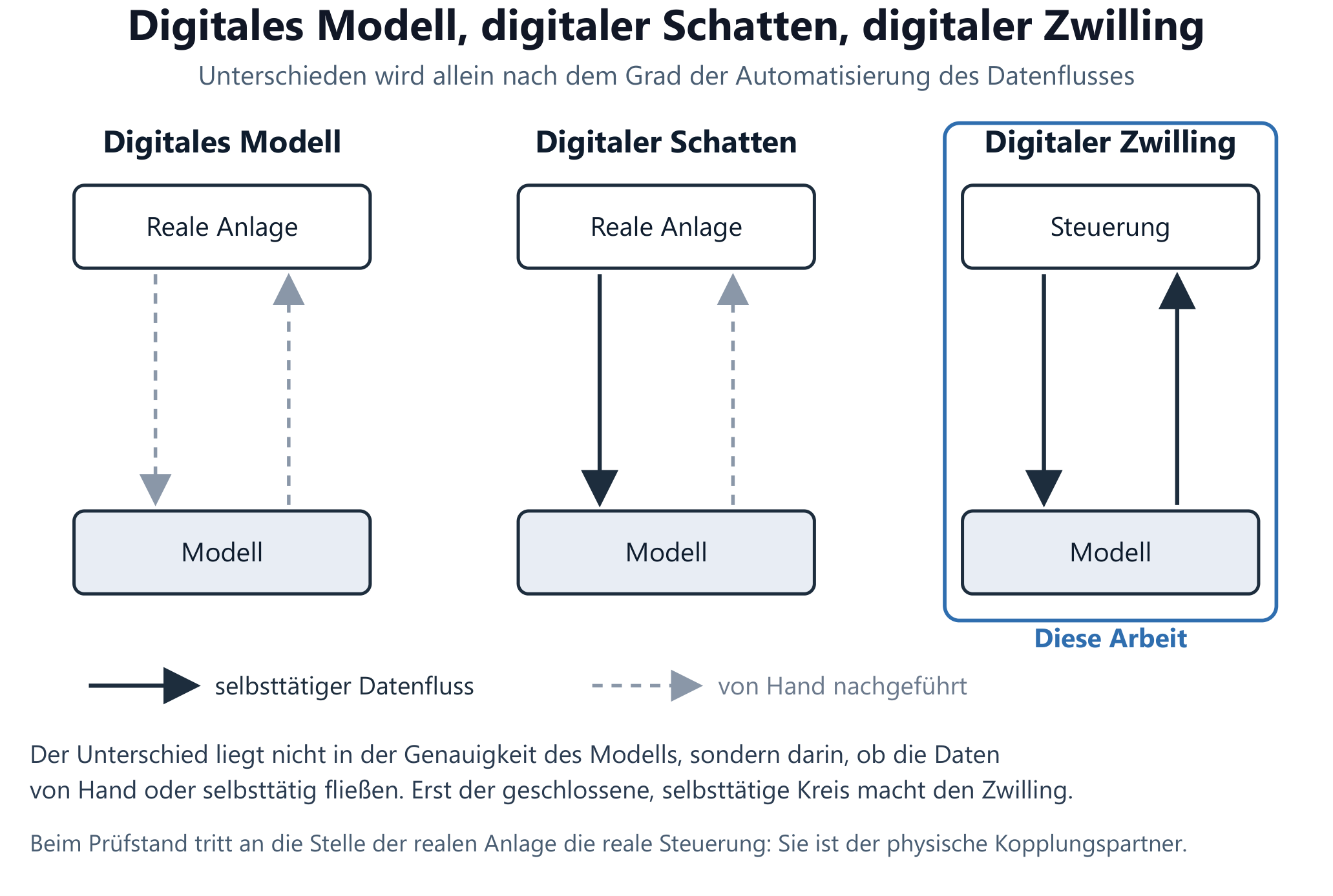
Model, shadow, twin
The distinction is made solely by the degree of automation of the data flow — this thesis sits at the twin.
-
Fig. 17
Signal direction
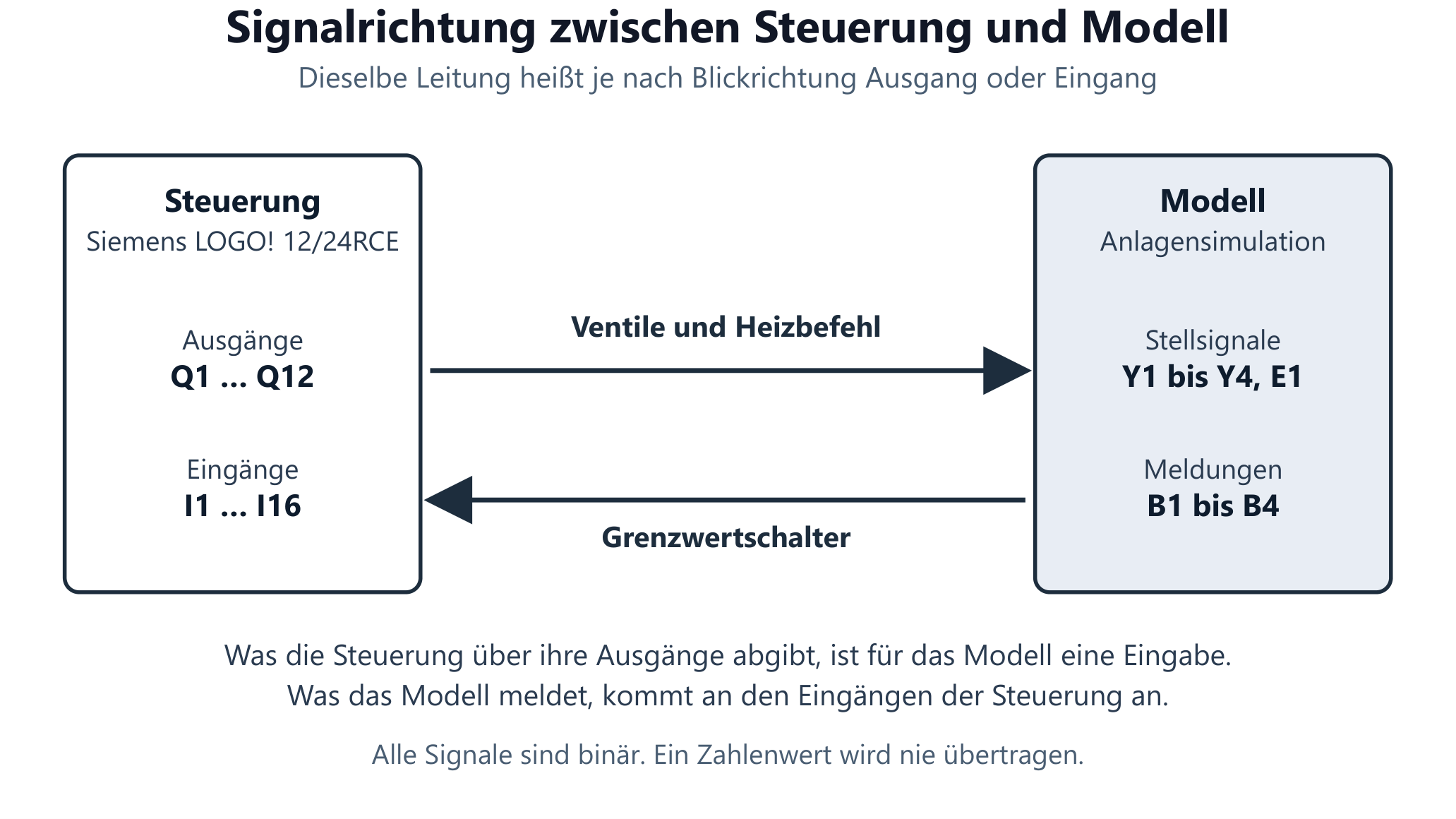
Depending on the viewing direction, the same line is called output or input: actuating signals Y1–Y4 and E1 forward, sensors B1–B4 back.
-
Fig. 18
System boundary
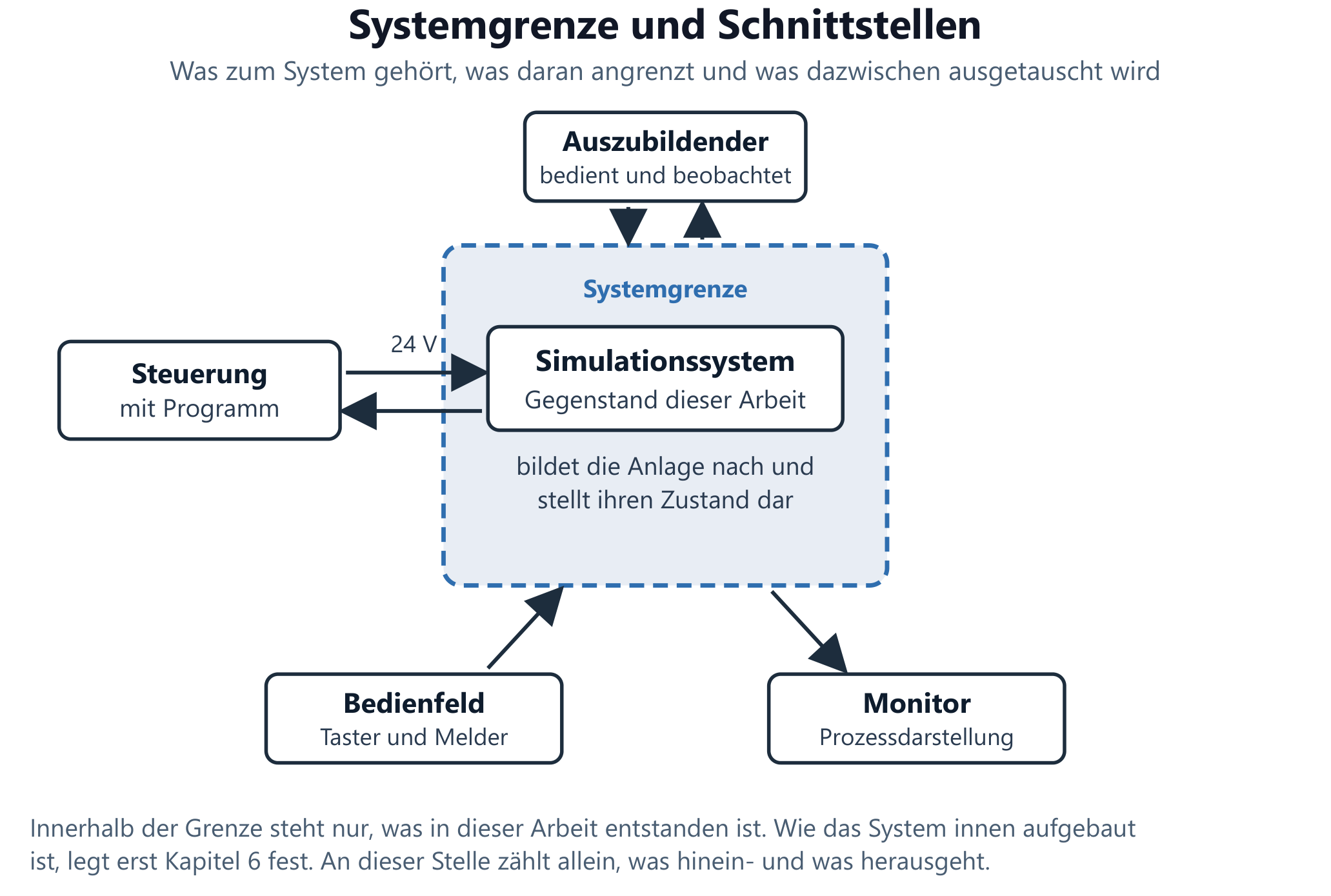
What belongs to the system, what adjoins it and what is exchanged in between.
-
Test plot 1
Filling
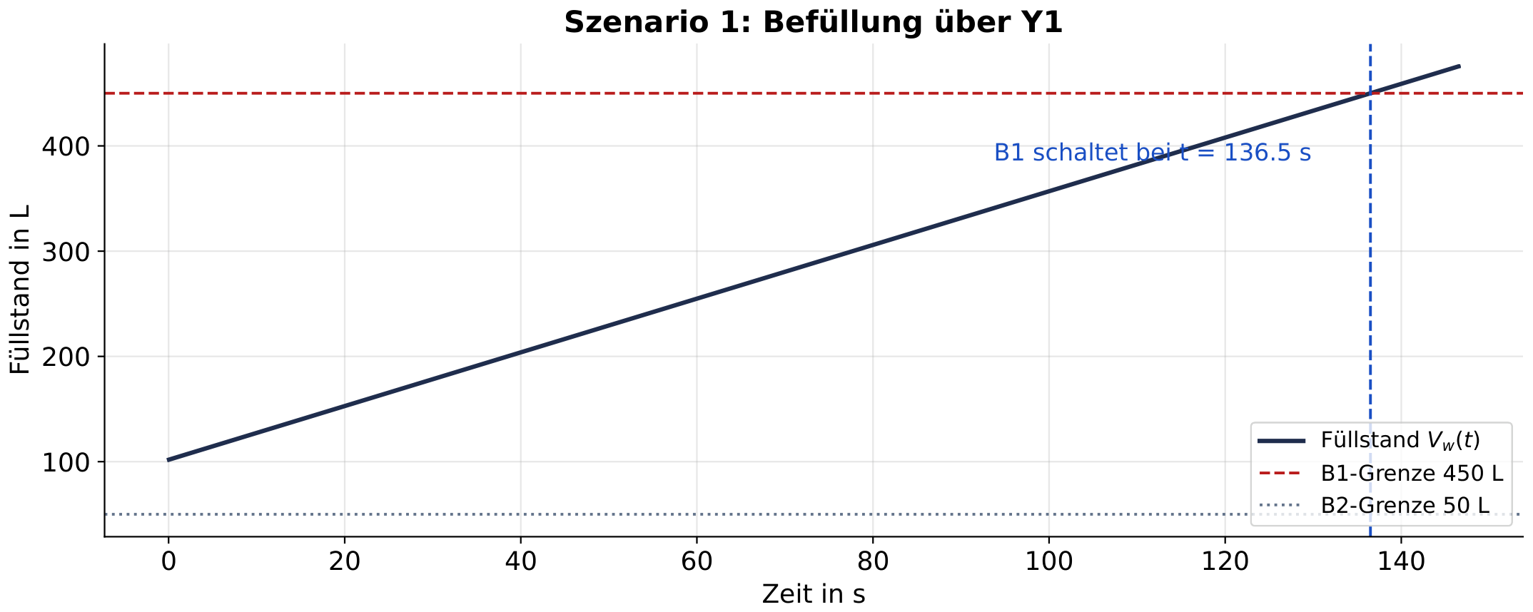
Fill level curve during filling up to the B1 report at t = 136.5 s.
-
Test plot 2
Heating
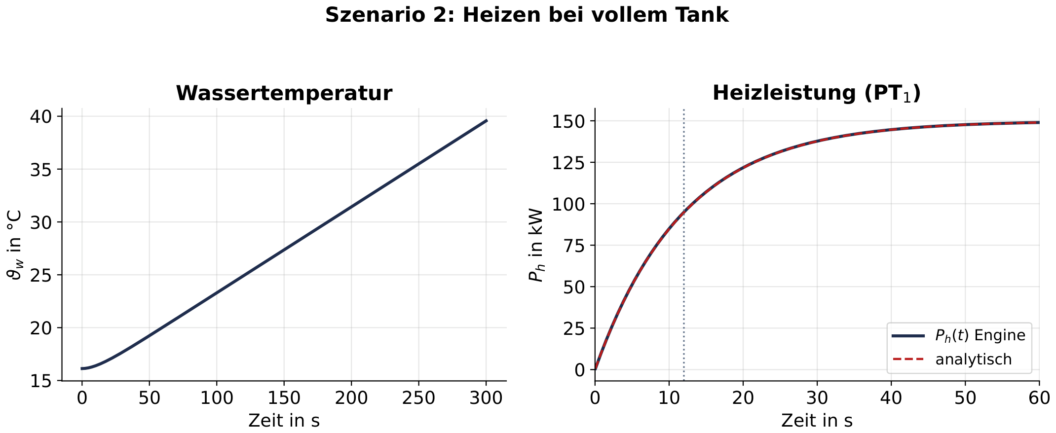
Calculated heating power of the model against the analytical PT1 solution (right) and water temperature over 300 s (left).
-
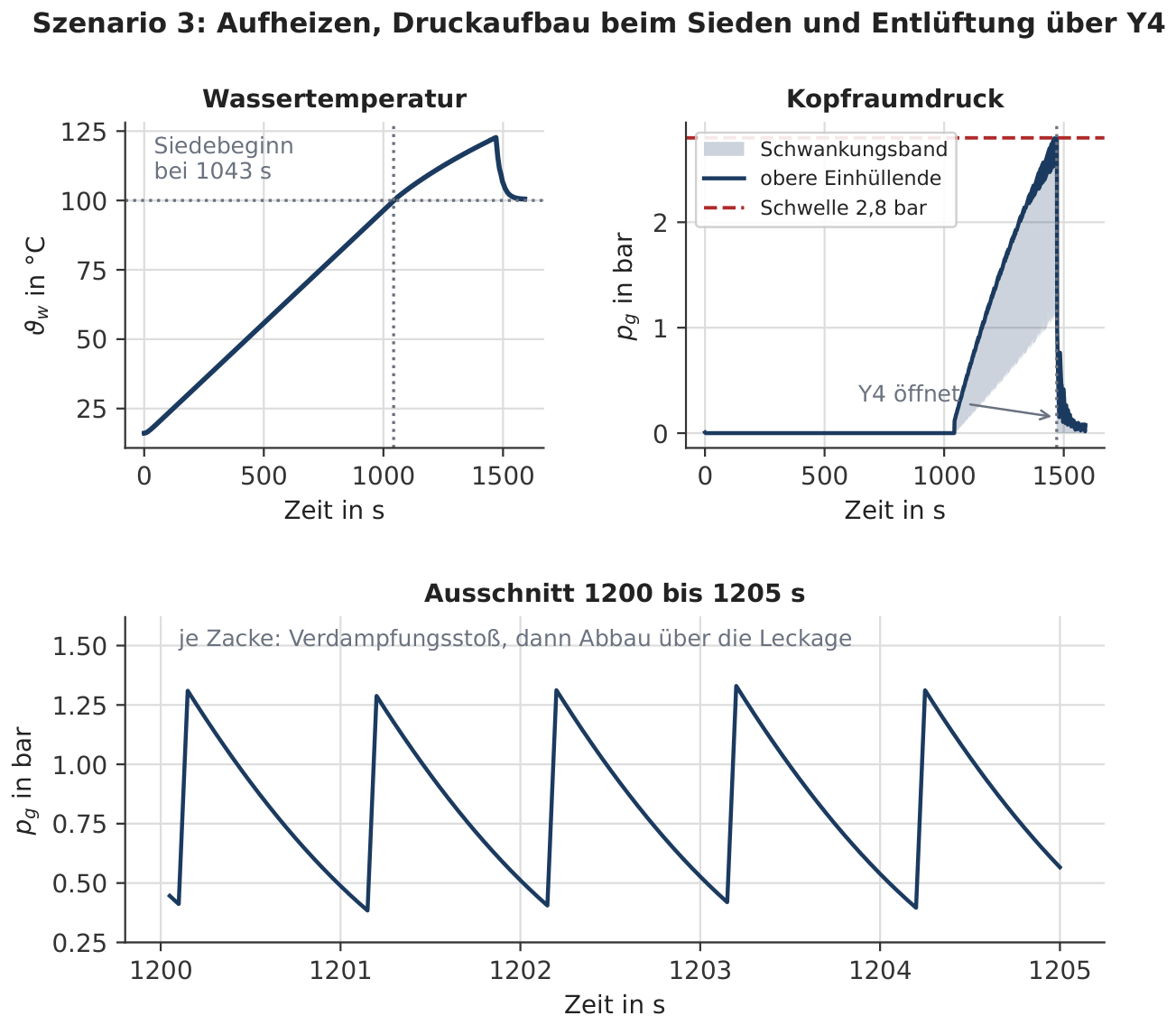
Test plot 3
Pressure build-up
Temperature and pressure curve up to the alarm threshold B4 and then venting via Y4; the headspace pressure fluctuates in a sawtooth pattern (fluctuation band).
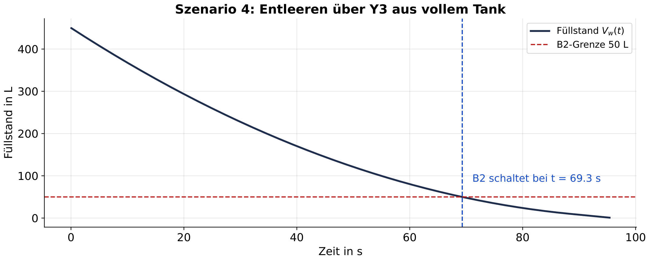
-
Test plot 4
Draining
Fill level during draining via Y3 from a full tank until empty; B2 switches at t = 69.3 s. The expected duration of 96.1 s is given in the test table.
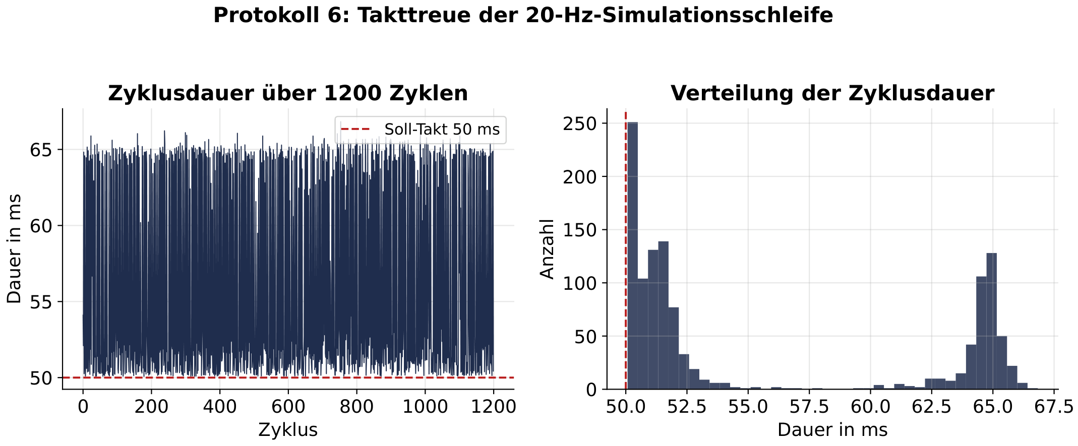
-
Test plot 6
Cycle adherence
Cycle duration of the simulation loop over 1200 cycles against the target cycle of 50 ms, plus the distribution of the cycle duration.
-
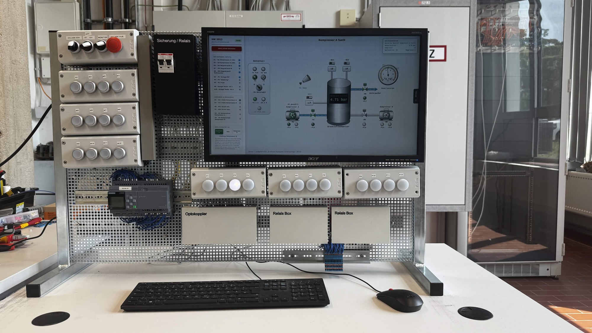
Photo
Test rig — front
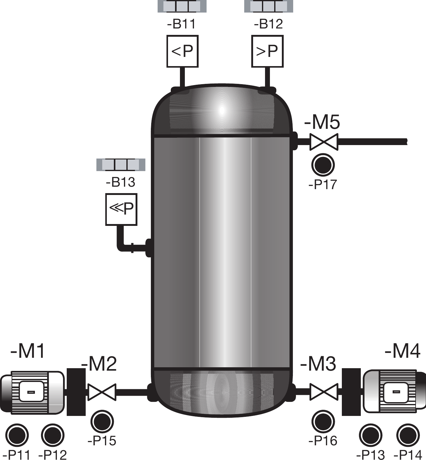
Controller, control panel with 12 push buttons and indicator lights, and the screen with a running simulation (the picture shows the compressed-air plant).
-
Photo
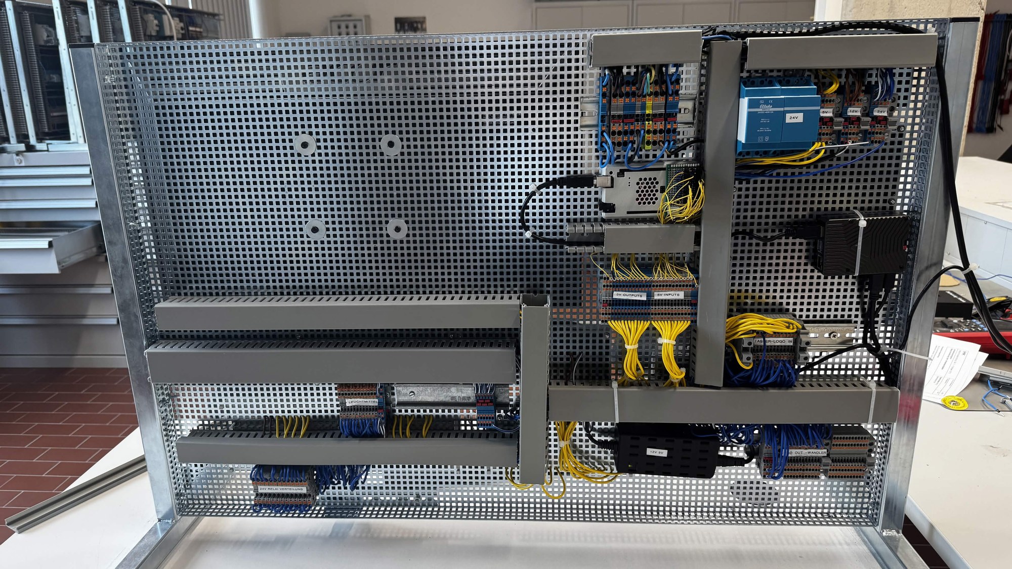
Test rig — back
Wiring of the signal level: power supplies, optocoupler assembly, relay board and signal bridge.
-
Photo
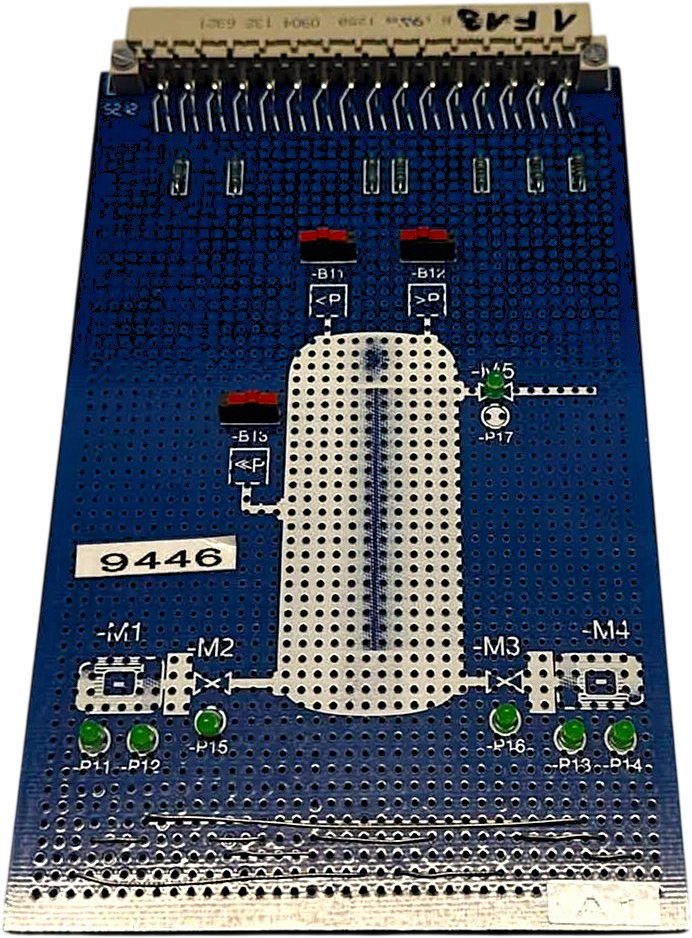
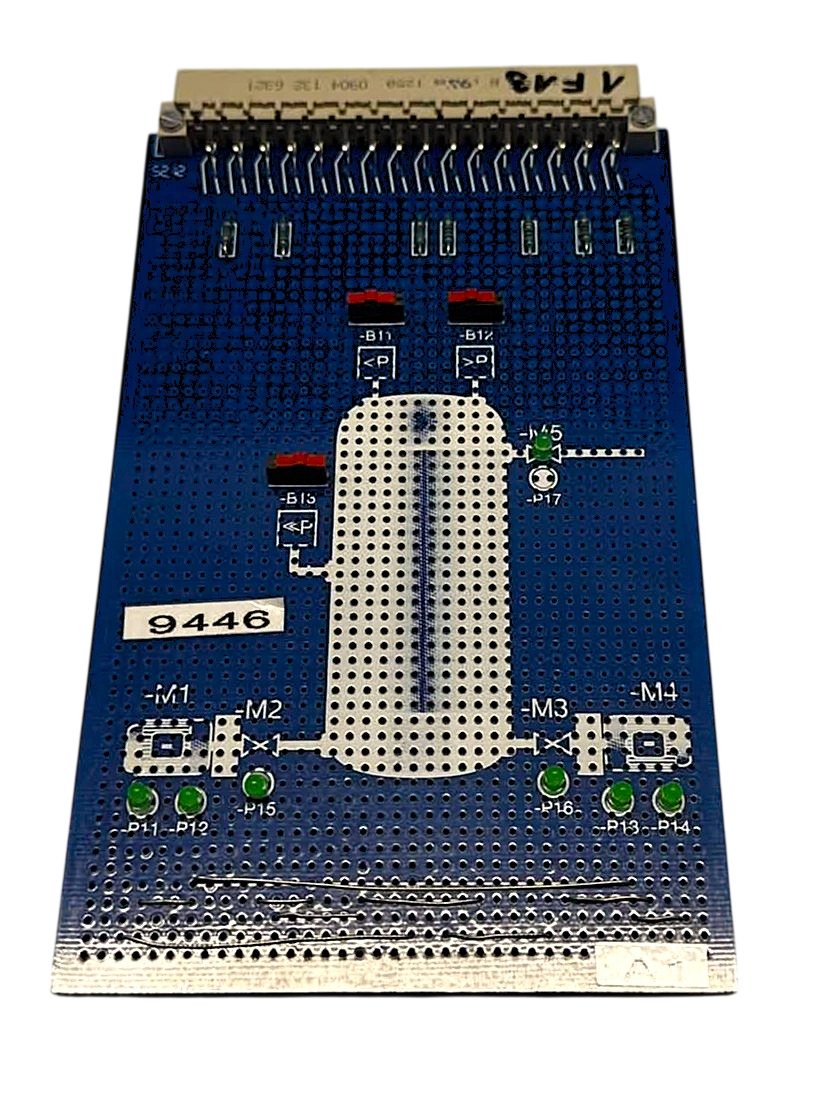
Preliminary project — compressed-air assembly
Board of the compressed-air control from the IHK project.
-
Photo
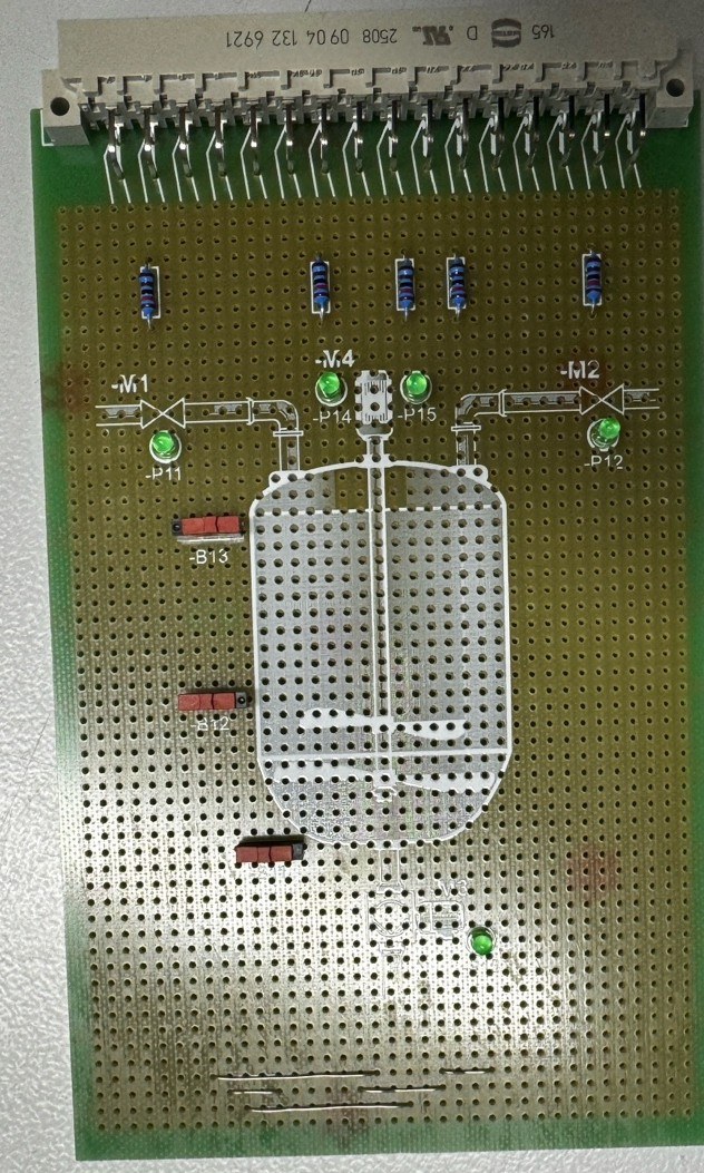
Preliminary project — board (photo)
Assembled assembly from the IHK project before the bachelor's thesis.
-
Circuit diagram & layout
Preliminary project — board layout
Layout of the same assembly.
-
Circuit diagram & layout
Preliminary project — compressed-air schematic
Circuit schematic of the compressed-air control from the IHK project.

No figure matches this selection.